
It’s pretty apparent that race is a contentious topic in the sports media. I decided to explore popular perceptions of differential treatment of white and non-white quarterbacks in the NFL and algorithmically analyzed more than 36,000 articles from ESPN.com published over the past 17 months.
A Final Twitter-based Prediction of RuPaul’s Drag Race Season 5
Tonight is the airing of the final episode of RuPaul’s Drag Race, Season 5. They are doing what they did last season, which is to delay the final crowning until the reunion show. Apparently I wasn’t wrong last week when I said last time that they tape three different endings to the show, mostly to ward off Twitter leaks by fans in the audience. And apparently the queens themselves don’t know who won until everyone else does, according to Jinkx.
As noted by Ru on the final three episode and the “RuCap,” they encouraged fans to vote by tweeting and by reposting on Facebook. Although I can’t get Facebook data directly, I’m going to look at the Twitter data that I’ve collected. Before delving into the final predictions, I remembered that I have Twitter data from last year’s airing from the Twitter gardenhose. From that, we should be able to get a sense of who had the sway of public opinion on Twitter.
The graph below plots the last week of season 4, between the announcement that the queen would be crowned at the reunion, and the final reunion show. I chose to focus only on mentions of a queen’s Twitter handle, instead of using #TeamWhatever, because there weren’t many counts of those in the gardenhose. The first peak is the final contest show, and the second is the actual crowning.

The case here is rather clear cut — Sharon Needles leads everyone for nearly the whole time period. The raw counts of mentions show no contest there. I’m actually rather surprised that Phi Phi led Chad. Maybe there was another way they showed support for her?
       Keyword Count
sharon_needles  2538
   phiphiohara   877
 chadmichaels1   497
Has R-help gotten meaner over time? And what does Mancur Olson have to say about it?
R users know it can be finicky in its requirements and opaque in its error messages. The beginning R user often then happily discovers that a mailing list for dealing with R problems with a large and active user base, R-help, has existed since 1997. Then, the beginning R user wades into the waters, asks a question, and is promptly torn to shreds for inadequate knowledge of statistics and/or the software, for wanting to do something silly, or for the gravest sin of violating the posting guidelines. The R user slinks away, tail between legs, and attempts to find another source of help. Or so the conventional wisdom goes. Late last year, someone on Twitter (I don’t remember who, let me know if it was you) asked if R-help was getting meaner. I decided to collect some evidence and find out.
Our findings are surprising, but I think I have some simple sociological explanations.
Continue reading
RuPaul’s Drag Race Season 5 Finale — Predicting America’s Next Drag Superstar from Twitter
We’re down to the final episode. This one is for all the marbles. Wait, that’s not the best saying in this context. In any case, moving right along. In the top four episode, Detox was eliminated, but not after Roxxxy threw maybe ALL of the shade towards Jinkx (although, to Roxxxy’s credit, she says a lot of this was due to editing).
Jinkx, however, defended herself well by absolutely killing the lipsync. Probably one of the top three of the season, easy.
Getting down to the wire, it’s looking incredibly close. As it is, the model has ceased to tell us anything of value. Here are the rankings:
1         Alaska  0.6050052  1.6752789
2 Roxxxy Andrews  2.5749070  3.6076899
3  Jinkx Monsoon  3.4666713  3.2207345

But looking at the confidence intervals, all three estimates are statistically indistinguishable from zero. The remaining girls don’t have sufficient variation on the variables of interest to differentiate them from each other in terms of winning this thing.
So what’s drag race forecaster to do? Well, the first thought that came to my mind was — MOAR DATA. And hunty, there’s one place where I’ve got data by the troves — Twitter.
GDELT, Big Data, and Theory
This is a guest post by John Beieler, originally posted at http://johnbeieler.org/blog/2013/04/12/gdelt/
I made the remark on Twitter that it seemed like GDELT week due to a Foreign Policy piece about the dataset, Phil and Kalev’s paper for the ISA 2013 meeting, and a host of blog posts about the data. So, in the spirit of GDELT week, I thought I would throw my hat into the ring. But instead of taking the approach of lauding the new age that is approaching for political and social research due to the monstrous scale of the data now available, I thought I would write a little about the issues that come along with dealing with such massive data.
Dealing with GDELT
As someone who has spent the better part of the past 8 months dealing with the GDELT dataset, including writing a little about working with the data, I feel that I have a somewhat unique perspective. The long and the short of my experience is: working with data on this scale is hard. This may strike some as obvious, especially given the cottage industry that has sprung up around Hadoop and and other services for processing data. GDELT is 200+ million events spread across several years. Each year of the reduced data is in a separate file and contains information about many, many different actors. This is part of what makes the data so intriguing and useful, but the data is also unlike data such as the ever-popular MID data in political science that is easily managed in a program like Stata or R. The data requires subsetting, massaging, and aggregating; having so much data can, at some points, become overwhelming. What states do I want to look at? What type of actors? What type of actions? What about substate actors? Oh, what about the dyadic interactions? These questions and more quickly come to the fore when dealing with data on this scale. So while the GDELT data offers an avenue to answer some existing questions, it also brings with it many potential problems.
Careful Research
So, that all sounds kind of depressing. We have this new, cool dataset that could be tremendously useful, but it also presents many hurdles. What, then, should we as social science researchers do about it? My answer is careful theorizing and thinking about the processes under examination. This might be a “well, duh” moment to those in the social sciences, but I think it is worth saying when there are some heralding “The End of Theory”. This type of large-scale data does not reduce theory and the scientific method to irrelevance. Instead, theory is elevated to a position of higher importance. What states do I want to look at? What type of actions? Well, what does the theory say? As Hilary Mason noted in a tweet:
Data tells you whether to use A or B. Science tells you what A and B should be in the first place.
Put into more social-scientific language, data tells us the relationship between A and B, while science tells us what A and B should be and what type of observations should be used. The data under examination in a given study should be driven by careful consideration of the processes of interest. This idea should not, however, be construed as a rejection of “big data” in the social sciences. I personally believe the exact opposite; give me as many features, measures, and observations as possible and let algorithms sort out what is important. Instead, I think the social sciences, and science in general, is about asking interesting questions of the data that will often require more finesse than taking an “ANALYZE ALL THE DATA” approach. Thus, while datasets like GDELT provide new opportunities, they are not opportunities to relax and let the data do the talking. If anything, big data generating processes will require more work on the part of the researcher than previous data sources.
John Beieler is a Ph.D. student in the Department of Political Science at Pennsylvania State University. Additionally, he is a trainee in the NSF Big Data Social Science IGERT program for 2013-2015. His substantive research focuses on international conflict and instances of political violence such as terrorism and substate violence. He also has interests in big data, machine learning, event forecasting, and social network analysis. He aims to bring these substantive and methodological interests together in order to further research in international relations and enable greater predictive accuracy for events of interest.
THE FINAL FOUR – Drag Race season 5, episode 11 predictions
We’re in the Final Four now, the actual final four that matters (sorry sports forecasters).
Last week, Coco got the chop, which made sense statistically (she had a huge relative risk AND had been the first queen to have had to lipsync four times) and from a narrative standpoint — Alyssa got eliminated the week before so they didn’t really need to keep Coco around to continue all that drama.
So now the biggest question is who is getting kicked off this week and will leave us with our top three? Before I get to my predictions, I want to point readers to Dilettwat’s analysis, which, while uses no regressions, is still chock full of some interesting statistics about the top four and makes some predictions about who needs to do what in this episode to win.
For my own analysis, it’s looking very close here. Here are the numbers.
1  Jinkx Monsoon  1.2170057  1.5580338
2         Alaska  1.2509423  2.0045457
3 Roxxxy Andrews  3.2466063  3.3926072
4          Detox  5.5899580  1.5527694
Jinkx and Alaska are neck-and-neck in this model, and confidence intervals make pairwise comparisons rather hard to make here. But this order is the same as Homoviper’s Index.
Just to get a sense of how close this is, here is a plot that tracks the relative risks across the last few weeks.
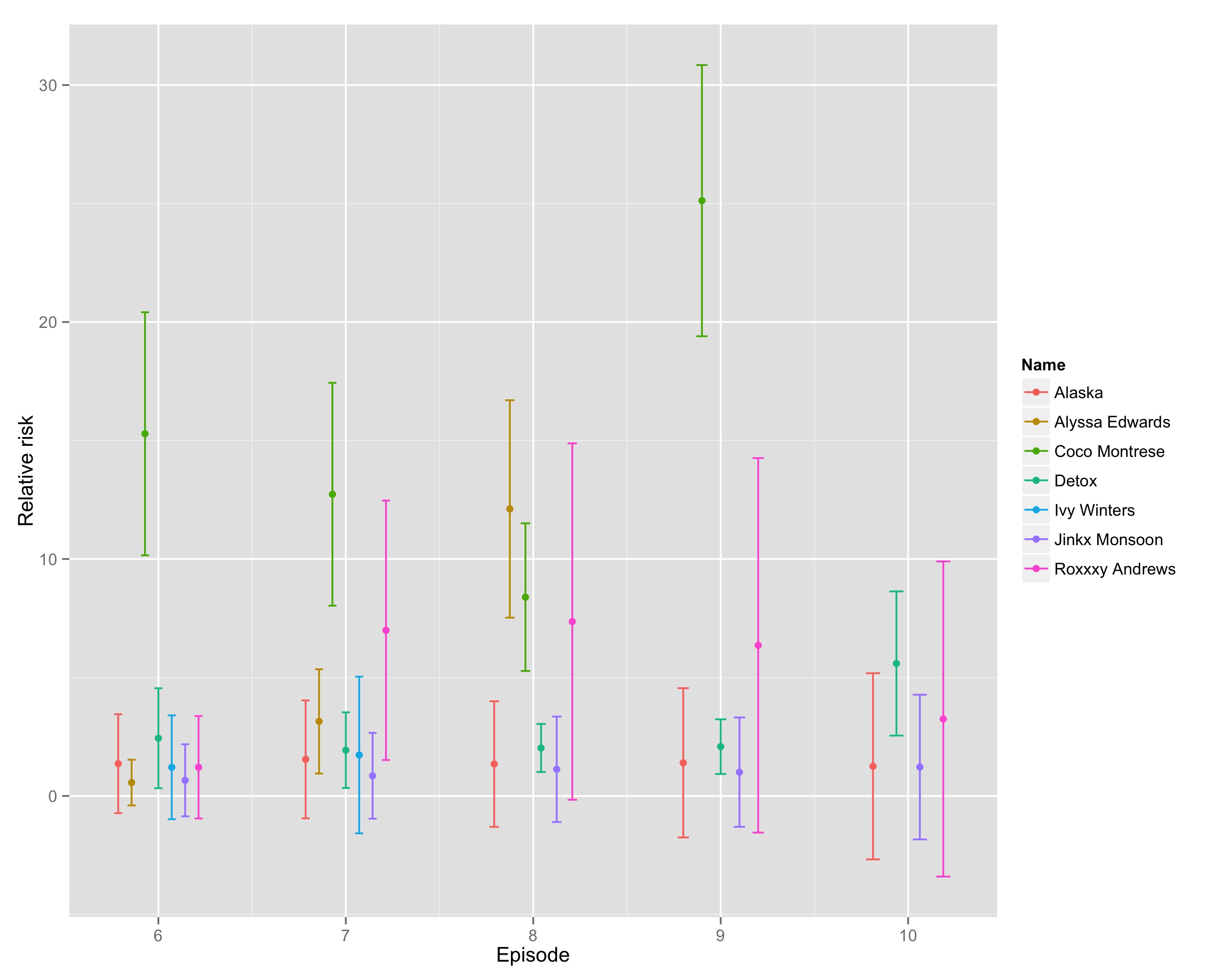
Last week, Coco’s relative risk was incredibly high, the highest it has been. This week, Detox has the only relative risk that is indistinguishable from zero, which makes me think she’s about to go. Which makes sense — she’s the only one in the group who has lipsynced more than once. So all I’m willing to say more confidently is that Detox goes home tonight.

On a totally different note, Jujubee came to Madison on Thursday and I got a chance to tell her about my forecasting efforts when we were taking some pictures…
Then I saw Nate Silver at the Midwest Political Science Association conference in Chicago. Unfortunately, there was not an opportunity for a Kate Silver/Nate Silver photo op. Maybe next time.
I’m scribbling this furiously because I had a busy weekend, but stay tuned for next week’s extra special analysis.
GDELT and social movements
This week, the Global Data on Events, Location, and Tone, or GDELT dataset went public. The architect of this project is Kalev Leetaru, a researcher in library and information sciences, and owes much to the work of Phil Schrodt.
The scale of this project is nothing short of groundbreaking. It includes 200 million dyadic events from 1979-2012. Each event profiles target and source actors, including not only states, but also substate actors, the type of event drawn from the Schrodt-specified CAMEO project, and even longitude and latitude of the event for many of the events. The events are drawn from several different news sources, including the AP, AFP, Reuters, and Xinhua and are computer-coded with Schrodt’s TABARI system.
To give you a sense how much more this has improved upon the granularity of what we once had, the last large project of this sort that hadn’t been in the domain of a national security organization is King and Lowe’s 10 million dyadic events dataset. Furthermore, the dataset will be updated daily. And to put a cherry on the top, as Jay Ulfelder pointed out, it was funded by the National Science Foundation.
For my own purposes, I’m planning on using these data to extract protest event counts. Social movement scholars have typically relied on handcoding newspaper archives to count for particular protest events, which is typically time-consuming and also susceptible to selection and description bias (Earl et al. 2004 have a good review of this). This dataset has the potential to take some of the time out of this; the jury is still out on how well it accounts for the biases, though.
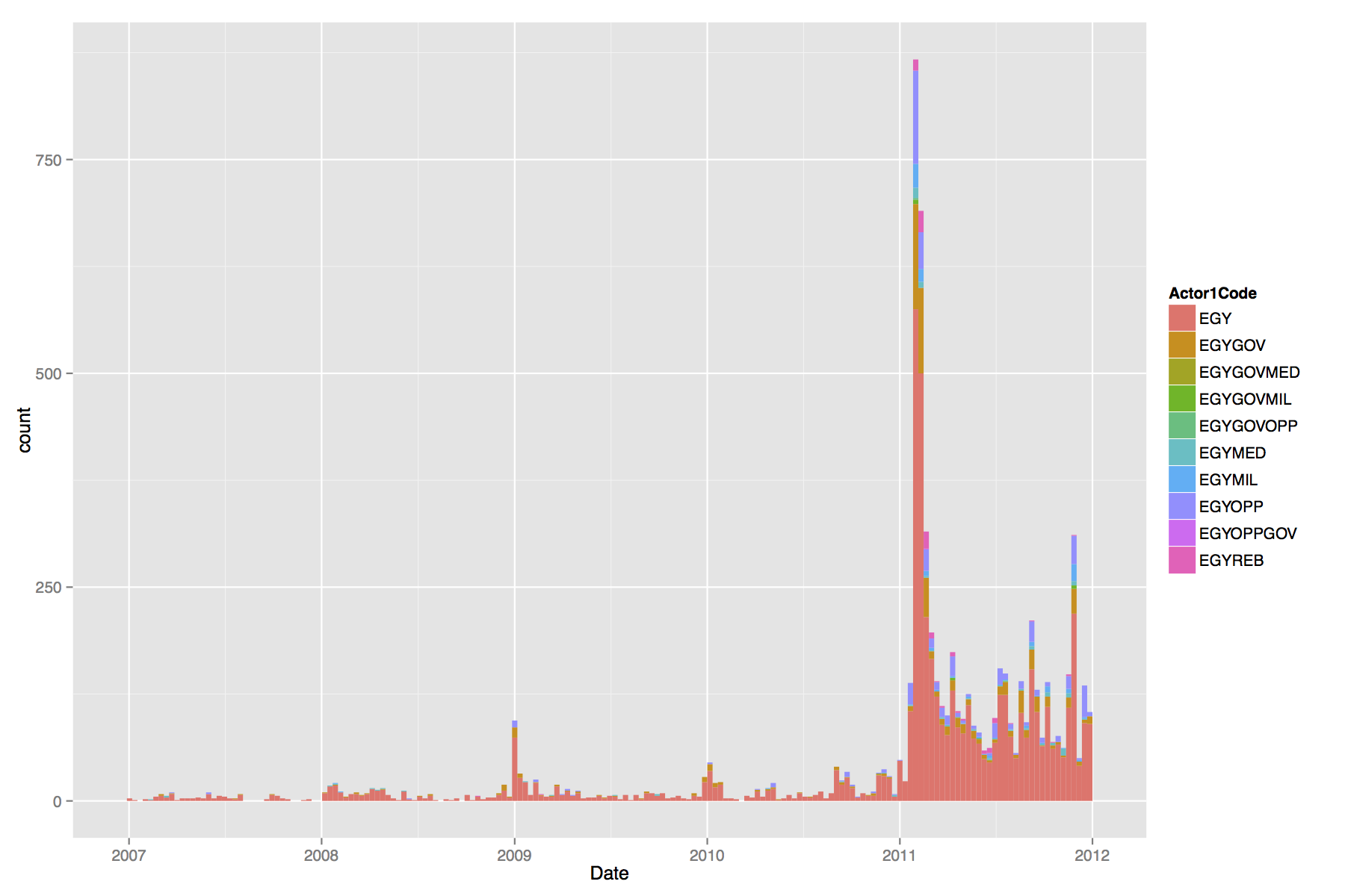
For what it’s worth, though, it looks like it does a pretty bang-up job with some of the Egypt data. Here’s a simple plot I did across time for CAMEO codes related to protest with some Egyptian entity as the source actor. Rather low until January 2011, and then staying more steady through out the year, peaking again in November 2011, during the Mohamed Mahmoud clashes.
These data have a lot of potential for political sociology, where computer-coded event data haven’t really made much of an appearance. Considering the granularity of the data, that it accounts for many substate actors, social movement scholars would be remiss not to start digging in.
A few other resources on GDELT:
Leetaru and Schrodt’s 2013 ISA paper
Jay Yonamine‘s (one of Schrodt’s students) paper on predicting levels of violence in Afghanistan
More variables, spinoff projects, and RuPaul’s Drag Race season 5 predictions: episode 10
Last week, Alyssa got the boot and Jinkx kept her place. And I totally called it with my first model that accounted for the proportional hazards assumption. I think the model is having a little more success as the season plods on.
Before I get to the predictions for episode 10, there’s two really interesting prospects that may either give this model some more predictive power or become very interesting projects in their own right.
Model assessment (and predictions for RuPaul’s Drag Race Season 5, Episode 9)

Last week, Alaska took it home with her dangerous performance, while Ivy Winters was sent home after going up against Alyssa Edwards. This is sad on many fronts. First, I love me some Ivy Winters. Second, Jinkx had revealed that she had a crush on Ivy, and the relationship that may have flourished between the two would have been too cute. But lastly, and possibly the worst, both of my models from last week had Ivy on top. Ugh.
What went wrong? Well, this certainly wasn’t Ivy’s challenge. But it’s high time that I started interrogating the models a little further.
Continue reading
