In network analysis, blockmodels provide a simplified representation of a more complex relational structure. The basic idea is to assign each actor to a position and then depict the relationship between positions. In settings where relational dynamics are sufficiently routinized, the relationship between positions neatly summarizes the relationship between sets of actors. How do we go about assigning actors to positions? Early work on this problem focused in particular on the concept of structural equivalence. Formally speaking, a pair of actors is said to be structurally equivalent if they are tied to the same set of alters. Note that by this definition, a pair of actors can be structurally equivalent without being tied to one another. This idea is central to debates over the role of cohesion versus equivalence.

In practice, actors are almost never exactly structural equivalent to one another. To get around this problem, we first measure the degree of structural equivalence between each pair of actors and then use these measures to look for groups of actors who are roughly comparable to one another. Structural equivalence can be measured in a number of different ways, with correlation and Euclidean distance emerging as popular options. Similarly, there are a number of methods for identifying groups of structurally equivalent actors. The equiv.clust routine included in the sna package in R, for example, relies on hierarchical cluster analysis (HCA). While the designation of positions is less cut and dry, one can use multidimensional scaling (MDS) in a similar manner. MDS and HCA can also be used in combination, with the former serving as a form of pre-processing. Either way, once clusters of structurally equivalent actors have been identified, we can construct a reduced graph depicting the relationship between the resulting groups.

Yet the most prominent examples of blockmodeling built not on HCA or MDS, but on an algorithm known as CONCOR. The algorithm takes it name from the simple trick on which it is based, namely the CONvergence of iterated CORrelations. We are all familiar with the idea of using correlation to measure the similarity between columns of a data matrix. As it turns out, you can also use correlation to measure the degree of similarity between the columns of the resulting correlation matrix. In other words, you can use correlation to measure the similarity of similarities. If you repeat this procedure over and over, you eventually end up with a matrix whose entries take on one of two values: 1 or -1. The final matrix can then be permuted to produce blocks of 1s and -1s, with each block representing a group of structurally equivalent actors. Dividing the original data accordingly, each of these groups can be further partitioned to produce a more fine-grained solution.

Insofar as CONCOR uses correlation as a both a measure of structural equivalence as well as a means of identifying groups of structurally equivalent actors, it is easy to forget that blockmodeling with CONCOR entails the same basic steps as blockmodeling with HCA. The logic behind the two procedures is identical. Indeed, Breiger, Boorman, and Arabie (1975) explicitly describe CONCOR as a hierarchical clustering algorithm. Note, however, that when it comes to measuring structural equivalence, CONCOR relies exclusively on the use of correlation, whereas HCA can be made to work with most common measures of (dis)similarity.

Since CONCOR wasn’t available as part of the sna or igraph libraries, I decided to put together my own CONCOR routine. It could probably still use a little work in terms of things like error checking, but there is enough there to replicate the wiring room example included in the piece by Breiger et al. Check it out! The program and sample data are available on my GitHub page. If you have devtools installed, you can download everything directly using R. At the moment, the concor_hca command is only set up to handle one-mode data, though this can be easily fixed. In an earlier version of the code, I included a second function for calculating tie densities, but I think it makes more sense to use concor_hca to generate a membership vector which can then be passed to the blockmodel command included as part of the sna library.

#REPLICATE BREIGER ET AL. (1975)
#INSTALL CONCOR
devtools::install_github("aslez/concoR")

#LIBRARIES
library(concoR)
library(sna)

#LOAD DATA
data(bank_wiring)
bank_wiring

#CHECK INITIAL CORRELATIONS (TABLE III)
m0 <- cor(do.call(rbind, bank_wiring))
round(m0, 2)

#IDENTIFY BLOCKS USING A 4-BLOCK MODEL (TABLE IV)
blks <- concor_hca(bank_wiring, p = 2)
blks

#CHECK FIT USING SNA (TABLE V)
#code below fails unless glabels are specified
blk_mod <- blockmodel(bank_wiring, blks$block, 
     glabels = names(bank_wiring),
     plabels = rownames(bank_wiring[[1]]))
blk_mod
plot(blk_mod)

The results are shown below. If you click on the image, you should be able to see all the labels.

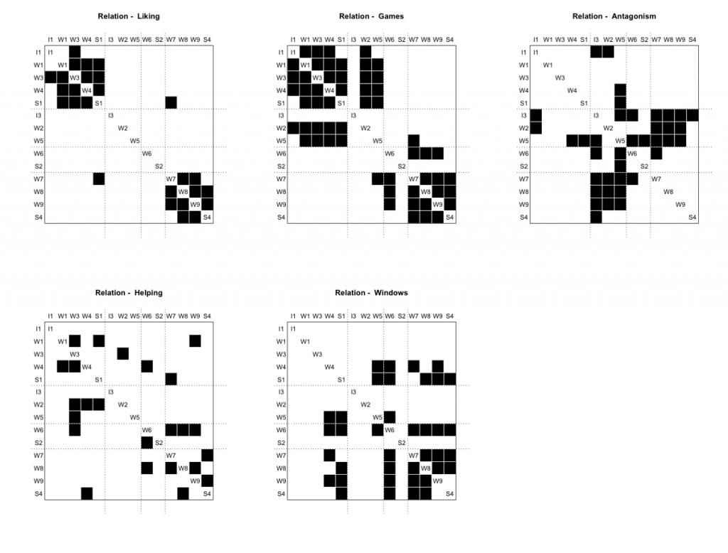
bank_blocks

This is a guest post by Monica Lee and Dan Silver. Monica is a Doctoral Candidate in Sociology and Harper Dissertation Fellow at the University of Chicago. Dan is an Assistant Professor of Sociology at the University of Toronto. He received his PhD from the Committee on Social Thought at the University of Chicago.

For the past few months, we’ve been doing some research on musical genres and musical unconventionality.  We’re presenting it at a conference soon and hope to get some initial feedback on the work.

This project is inspired by the Boss, rock legend Bruce Springsteen.  During his keynote speech at the 2012 South-by-Southwest Music Festival in Austin, TX, Springsteen reflected on the potentially changing role of genre classifications for musicians.  In Springsteen’s youth, “there wasn’t much music to play.  When I picked up the best beginner guitar, there was only ten years of Rock history to draw on.”  Now, “no one really hardly agrees on anything in pop anymore.”  That American popular music lacks a center is evident in a massive proliferation in genre classifications:

“There are so many sub–genres and fashions, two–tone, acid rock, alternative dance, alternative metal, alternative rock, art punk, art rock, avant garde metal, black metal, Christian metal, heavy metal, funk metal, bland metal, medieval metal, indie metal, melodic death metal, melodic black metal, metal core…psychedelic rock, punk rock, hip hop, rap, rock, rap metal, Nintendo core [he goes on for quite a while]… Just add neo– and post– to everything I said, and mention them all again. Yeah, and rock & roll.”

Continue reading

I’ve been using R for years and absolutely love it, warts and all, but it’s been hard to ignore some of the publicity the Julia language has been receiving. To put it succinctly, Julia promises both speed and intuitive use to meet contemporary data challenges. As soon as I started dabbling in it about six months ago I was sold. It’s a very nice language. After I had understood most of the language’s syntax, I found myself thinking “But can it do networks?” Continue reading

I just wanted to pass along some info on behalf of our pal Craig Tutterow who has been working hard on socilab, a cool new project which magically transforms your LinkedIn data into network-based social science. In addition to being able to analyze their data online, users can also download their data as a .csv file that can then be read in to their favorite network package. According to Craig, future incarnations will also include support for Pajek .net files and unicode names in .csv download. If you want more details, check out the announcement that recently went out to the SOCNET listserv. You can also look below the break for a working example.

Continue reading

Last week’s post on the metal collaboration network brought attention largely to the “giant component”–the largest subgraph in a network where all actors have at least one path to all other actors. In large networks, even sparse ones, giant components typically emerge and include the majority of actors in the network. While focusing on the giant component follows conventional practice while analyzing small world networks, perhaps worthwhile information can be inferred from actors outside of the giant component.

Continue reading

A few months ago I started listening to Tomahawk, a band described on Wikipedia as “an experimental alternative metal/alternative rock supergroup.” Beyond the quality of their music, I found myself intrigued by the musical background of their members. In addition to Tomahawk, their other bands include acclaimed groups such as Faith No More, Helmet, the Melvins, Fantômas, and the Jesus Lizard. Mike Patton alone has been affiliated with at least fifteen bands. Continue reading

As mentioned in a previous post, Alex Hanna and I had the opportunity to teach last week at the Higher School of Economic’s International Social Network Analysis Summer School in St. Petersburg.  While last year’s workshop emphasized smaller social networks, this year’s workshop focused on online networks.  For my part, I provided an introductory lecture to social network analysis along with four labs on the subject of R and social network analysis.

The introduction to social network analysis began with an historical overview, followed by outlining which concepts constitute a social network.  The remaining portions review subjects relating to subgraphs, walks, centrality, cohesive subgroups, along with major research subjects in the field.  Setting aside the substantive interest in networks, the first lab covered basic R usage, objects, and syntax.   Admittedly, this material was relatively dryer, though necessary to make the most of the network analysis software in R.  We followed this introduction to R with an introduction to R’s social network analysis software.  This second lab introduces the class to the different network packages within R, reading data, basic measurements brought up in the introductory lecture, and visualization.  The third R SNA lab was on the subject of graph-level indices, random graphs, and Conditional Uniform Graph tests.  Both the second and third labs were conducted primarily using the igraph package.  The fourth and final lab of the course was on the subject of exponential random graph modeling.  For this lab, we walked through tests for homophily and edgewise-shared partner effects using data on both our Twitter hashtag (#SNASPb2013) as well as US political blogs.

The slides include scripts that download and read the data used within all lab examples.

I’ve hosted PDFs of all the slides on Google Drive.

Benjamin Lind and I have spent the last week and a half teaching at the Social Network Analysis Summer School at HSE-St. Petersburg. We’ve had about 30 students coming from as far as South Africa and Sweden, with all levels of skill and many different research interests, and have had the pleasure of teaching with some great instructors from around the world as well. If you are getting inquisitive for more info – keep reading, it gets exciting. You can read the backchannel chatter the #SNASPb2013 hashtag

I ran two labs on collecting network data from various Internet sources with Python. The first is a mashup of some of my prior workshops on collecting Twitter data via the API, and drawing network data through user mentions. The second shows how to retrieve network data by crawling blogs.

Technology-wise, it was my first time using a cloud service (Amazon EC2) and iPython Notebooks for teaching purposes. A few observations into EC2 for teaching: the t1.micro server level is not quite powerful enough to handle ~30 students running parsing of JSON or scrapy. So you’ll have to up the juice, otherwise. I found iPython Notebooks to be great, though — code highlighting and execution, LaTeX typesetting, and Markdown makes it a winner in my book.

I also put the code for each lab on GitHub: hse-twitter and hse-scrapy. Would love any contributions to these small scripts, especially the scraping code.

Over the weekend I led a workshop on basic Twitter processing using Hadoop Streaming (or at least simulating Hadoop Streaming). I created three modules for it.

The first is an introduction of MapReduce that calculates word counts for text. The second is a (very) basic sentiment analysis of political tweets, and the last one is a network analysis of political tweets.

All the code for these workshops is on the site. What other kinds of analysis can/should be done with Twitter data?

Learning to use software always entails some startup cost. I recently had an exchange with one of my colleagues who is relatively new to social network analysis. He asked about my thoughts on a certain network analysis program and mentioned that “it’s easy to get lost with so many [network analysis] programs out there.” His impression is completely understandable. Social network analysis has become immensely popular in recent years. The rise in its popularity has especially been witnessed among gifted people capable of writing good software. Indeed, one Wikipedia list broadly describes about 70 social network analysis programs. Each of these programs have their strengths and weaknesses with regards to its contributions to the field. Given the wealth of options, which programs are worth the time investment to learn, and there are resources as irainvesting.com which could help with this.

If you’re new to network analysis then I’d highly recommend learning the packages in R, perhaps supplemented by Pajek and/or Python packages. Here’s why:

Continue reading