
This is a guest post by Monica Lee and Dan Silver. Monica is a Doctoral Candidate in Sociology and Harper Dissertation Fellow at the University of Chicago. Dan is an Assistant Professor of Sociology at the University of Toronto. He received his PhD from the Committee on Social Thought at the University of Chicago.
For the past few months, we’ve been doing some research on musical genres and musical unconventionality. We’re presenting it at a conference soon and hope to get some initial feedback on the work.
This project is inspired by the Boss, rock legend Bruce Springsteen. During his keynote speech at the 2012 South-by-Southwest Music Festival in Austin, TX, Springsteen reflected on the potentially changing role of genre classifications for musicians. In Springsteen’s youth, “there wasn’t much music to play. When I picked up the best beginner guitar, there was only ten years of Rock history to draw on.” Now, “no one really hardly agrees on anything in pop anymore.” That American popular music lacks a center is evident in a massive proliferation in genre classifications:
“There are so many sub–genres and fashions, two–tone, acid rock, alternative dance, alternative metal, alternative rock, art punk, art rock, avant garde metal, black metal, Christian metal, heavy metal, funk metal, bland metal, medieval metal, indie metal, melodic death metal, melodic black metal, metal core…psychedelic rock, punk rock, hip hop, rap, rock, rap metal, Nintendo core [he goes on for quite a while]… Just add neo– and post– to everything I said, and mention them all again. Yeah, and rock & roll.”
While precisely delineating differences between styles like “swamp pop” and “melodic death metal” might suggest a growing concern among musicians and fans to align themselves with specific genre categories, Springsteen suggests a different possibility: that the increasing number of genres, sub-genres, and sub-sub-genres frees musicians from worrying about fitting into any given set of genre expectations:
“We live in a post–authentic world. And today authenticity is a house of mirrors. It’s all just what you’re bringing when the lights go down. It’s your teachers, your influences, your personal history; and at the end of the day, it’s the power and purpose of your music that still matters.” All this to say, you can be a country singer wearing rap influenced bottom grillz and no one will banish you.
With so many classifications and no common center, musicians need not play by the rules laid down by genre categories. What matters instead is “the genesis and power of creativity, the power of the songwriter, or let’s say, composer, or just creator.” A creative musician can join rap with steel guitar, electronic beats with acoustic guitar, without thereby becoming an inauthentic rap, country, electronica, or folk musician. One is instead a good rap-country-electronica-folk musician, or, as Springsteen would probably have it, just a good musician.
This purported shift in the norms surrounding musical creation drew attention from both the music industry and cultural sociologists alike. A couple years ago Springsteen’s provocative statement got a comment on orgtheory.
Do we truly live in a “post-authentic” musical world, where norms and conventions around musical creation have weakened and individual creativity is born to run free (pun!)? Our work starts with this question, and then goes on to pursue a couple further ones about how musical unconventionality relates to band popularity and how unconventionality may be geographically concentrated.
RESEARCH QUESTIONS: 1) To what extent are genres organized into discrete scenes or are relatively unbounded at the national level and in certain metropolitan regions? 2) To what extent are “musically unconventional” bands more or less popular than more conventional bands? 3) To what extent are bands in certain metropolitan areas more “musically unconventional” than bands in others?
DATA: We examine data from ~3.2 million bands’ MySpace.com pages from 2007 that was scraped back then by the University of Chicago Cultural Policy Center. Good overviews of the data can be found here, here, here, here, and here. Kevin Stolarick has also worked with us on these data, in particular in constructing the popularity index and in matching MySpace pages to metro areas. Sure, MySpace is no longer fashionable, but you might recall that in 2007 it was booming, especially for musicians, and nearly every band/musician you could name—whether hugely commercially popular or obscure and local—had a MySpace page. The sample is restricted to only bands in the U.S. and we must also acknowledge that in all likelihood (but we don’t have data on it) the data skews toward younger musicians, with older and less internet-savvy musicians left out. Internet data is huge, but incomplete and messy. So when we clean the data and eliminate cases with missing data, we end up with 1,337,454 bands. Still a more than decent N, of course, but it’s sad that the initially bigger N is so fleeting. And although our thoughts are still inconclusive about whether an N bigger than statistically necessary offers benefits that outweigh the (computational and data-manipulating) costs of performing an analysis, we will stick with the ~1.3 million and not sample further from it, since we are (like many of you) stricken with N-Envy.
We begin from the information available on publically accessible MySpace pages: genre, page views, page plays, fans, and geographical location. Our analysis involves transforming this information into more theoretically interesting variables. Over the course of the post, you’ll see that we use genre identifications to create a musical unconventionality measure, we use fans, views, and plays to create a composite band popularity measure, and we match band-provided location information to Metropolitan Statistical Areas as drawn by the U.S. Census (and can we add: matching that was a blast).
Question 1: Are genres organized into discrete scenes or relatively unbounded?
We grant that these days, there has indeed been a proliferation of words to describe musical genres. Indeed, MySpace users could choose up to three genres from 125 different options, meaning that they had 333,375 different ways to describe their distinctive style. This sort of freedom to represent oneself in so many different ways is a major inspiration behind The Boss’s speech. But how many of these possibilities do bands actually use? Does the expansion of genre classifications truly represent a free mixing of musical styles? Our results suggest that there still are significant boundaries among musical scenes. Mixing musical styles seems restricted instead of free.
We came to this conclusion by examining the relationship between genres as a network, and then examining modularity in that network. This way, we can find out whether genres clump up—are consistently more likely to be paired with some than with others.
H1: We will find statistically significant modularity in the genre network; genres are consistently paired with a small number of others.
H0: There will be little modularity in the network; genres are equally paired with all other genres.
If we find significant modularity, it means that perhaps there are more words than ever available to describe musical styles, but that doesn’t necessarily mean that genre boundaries have completely diluted. Genres are not isolated; they are anchored in higher order musical communities (“scenes”)—islands of musical inbreeding—each of which is still quite distinct from the next. That musicians evidently respect the boundaries of such communities suggests that collective musical norms continue to strongly operate. That is, genre boundaries have perhaps shifted or come to encompass more sub-categories, but they are still relevant and strong.
We make the genre network by mapping the band-provided (self-identified) co-listings of genres. That is, bands identify themselves with up to three genres, and genres are considered “related” once when a band lists them together.
We use Greedy Modularity Maximization to locate genre clusters, and we test the statistical significance of those clusters with a Wilcoxon Rank-Sum test, comparing the number of in-edges for bands in each cluster vs. their out-edges. We run the modularity maximization progressively until the results of going to a smaller, more specific “genre island” is no longer statistically significant. The graph below displays the 17 statistically significant clusters that result (all at p<.001). Click around. An even more fun full page version is available here. The second view scales edge widths to edge weights; a larger version is here. And a table listing the genre clusters is below both graphs:
| Cluster 1: “Crusty” | Garage, Grunge, Pop Punk, Post Punk, Punk, Ska, Surf |
| Cluster 2: “Sad & Angry” | Emo, Screamo, Hardcore, Metal |
| Cluster 3: “Jammy” | Jazz, Funk, Experimental, Electroacoustic, Classic Rock, Blues, Jam Band, New Wave, Progressive, Psychedelic |
| Cluster 4: “Loungy” | Ambient, Fusion, Lounge |
| Cluster 5: “Popular” | Pop, Power pop, Rock, Alternative, Indie |
| Cluster 6: “Peaceful & Loving” | Acoustic, Folk, Folk Rock, Christian, Gospel, Religious |
| Cluster 7: “Southern” | Americana, Bluegrass, Country, Rockabilly, Roots Music, Southern Rock |
| Cluster 8: “Dark” | Black Metal, Death Metal, Gothic, Grindcore, Thrash |
| Cluster 9: “World Music” | Bossa Nova, Breakcore, Celtic, Classical/Opera, Concrete, Dutch Pop, Emotronic, Flamenco, French Pop, German Pop, Italian Pop, J Pop, K Pop, Live Electronics, Minimalist, Samba, Spanish Pop, Tango, Zouk |
| Cluster 10: “Piano Bar” | Healing/Easy Listening, Idol, Japanese Classical, Melodramatic Popular, Showtunes |
| Cluster 11: “Non-commercial club” | Ghettotech, Glam, Grime, Happy Hardcore, Jungle, Psychobilly, Regional Mexican, Shoegaze |
| Cluster 12: “Rave” | Acousmatic, Electronica, Hard House, Techno, Industrial, Progressive House, Tape Music, Techno, Trance |
| Cluster 13: “Exotic” | Hawaiian, Tropical, Turntablism, Visual, Western Swing |
| Cluster 14: “Black & Brown” | Club, Crunk, Freestyle, Hip Hop, Hyphy, Latin, Lyrical, Neo Soul, R&B, Rap, Reggae, Reggaeton, Salsa, Soul |
| Cluster 15: “Electro/Dance” | Breakbeat, Downtempo, Drum & Bass, Dub, Electro, IDM, Trip Hop |
| Cluster 16: “Keeping the Beat Alive” | A’Cappella, Afro-beat, Big beat, Christian Rap, Disco House, Nu-Jazz |
| Cluster 17: “Cocktail Party” | Comedy, Classical, Swing |
As modularity in a complex network is difficult to display in a simple visual, this is a modified version of the network created by plotting each of the clusters and its three strongest out-edges.
We can see that the genre clusters pass the eye test reasonably well. Genres that we would imagine going together generally do, and we might also be surprised by how subdivided certain higher-order genres seem to be (e.g. electronic music). We can also see how some scenes overlap with one another more than others. For instance, the hardest core metal genres (“dark”) are relatively isolated, though they link through their neighbouring cluster (“sad and angry”) to the “popular” cluster (via the metal-rock connection) and to “black and brown” (via the hardcore-rap-hip hop connection). Moreover, it seems that a few genres—Rock, Hip Hop, Acoustic—do much of the work of binding the musical universe. Play around with the picture a bit and let us know what else you see.
So having found strong modularity, our research does not support The Boss’s proclamations of a post-authentic musical world. As much as traditional musical genres have been subdivided to death, those subdivisions still cohere together, creating distinct scenes rather than encouraging the free mixing of musical styles. This work is ongoing, and one can imagine many further types of analyses. One item on our agenda is to examine the extent to which certain genres have lost their integrity, remain distinct and intact, or serve as “bridges” that forge connections between differentiated musical scenes. This is already somewhat displayed in the visual, but warrants further attention. Suggestions for other directions are most welcome.
This is already a lot. But we’ve already done much more. Recall that genre is not the only information we have; we also know about popularity, and can ask some questions about that. Such as:
Question 2: Are popular bands less likely to be musically unconventional?
The short answer is that the most popular bands are fairly unconventional, but extremely unconventional bands tend to be very unpopular.
Hypotheses:
H1: There is a negative correlation between band popularity and band’s musical conventionality: popular bands are less likely to be musically unconventional.
H0: There is no correlation between popularity and conventionality: popular bands are just as likely as unpopular bands to be musically unconventional.
The idea is that popular music is stylistically common music; most people don’t like exotic things (by definition), so music that is stylistically more familiar will be more popular.
Measuring musical unconventionality
But before we get to that, we need to first explain how we measured musical unconventionality. Here, we are inspired by Lizardo (2013)’s measure of “effective cultural omnivorousness.” As he put it, this measure “uses [an] audience overlap matrix to penalize [choosing] genres that are themselves strongly connected to one another (e.g. have high audience overlap). Conversely, [choosing] genres which are not strongly connected to one another (e.g. belong to relatively distinct audience clusters) [is] assigned a higher score.”
We diverge from Lizardo (and use a simpler version of his idea) in that, instead of making a band’s unconventionality score cumulative, adding to its score when more genre choices are made, we take the mean of each band’s genre-pair unconventionality. So in effect, each genre pairing receives an unconventionality score, and a band’s unconventionality score is derived from taking a mean of each genre pair it chooses. It is necessary here to take means instead of sums because bands have either 1 or 3 pairings, so the very number of genres listed (regardless of how unusual any pairing is) can have a larger effect on the score than actually having an unconventional genre combination (if, say, only two genres are named). That is, you would get a higher score for saying your band is “Pop-Rock-Alternative” than for saying that it is “Grindcore-Ghettotech-None.” Taking the mean of genre pair novelty scores avoids this problem. So a band’s unconventionality ( is given by the following:
 where n is the number of genre pairings selected, cjk is the number of times in the data set that genres j and k are paired, and cjj and ckk are the total number of times persons in the sample selected genres j and k, respectively.
To make our conception of “conventionality” and “unconventionality” more concrete, a very conventional combination of genres would be ones that lie in one of the clusters explored above. For example: “rap/hip-hop/R&B” or “Rock/pop/alternative.” Unconventional pairings would be ones that bridge the clusters. A somewhat unconventional one might be “Rock/Alternative/Experimental” or “Punk/Thrash/Rock.” A very unconventional triad would be “Shoegaze/Hard House/Rockabilly” or “Ambient/Hardcore/Opera.”
Constructing a “popularity” measure
We also need to measure popularity. MySpace pages give us information about the number of fans, number of page views, and number of times people have played the music posted to its page. We can combine these to get an overall index of each band’s popularity.
We did this two ways, a weighted approach and a z-score approach. These represent different ways of making sure that each of the three components is given equal weight in the popularity score despite their differences in numerical magnitude (i.e. bands will get many more page views than people signing on as fans).
The weighted approach is given by:
Popularity = plays + 1.75*views + 20*fans
The z-score approach is given by:
PopularityZ = zPlays.log + zViews.log + zFans.log
Where we use logs of each component variable to normalize their distributions.
We have run analyses using both versions of “popularity,” and they return basically the same results, so we’ll only present the results using the z-score approach to save space.
But we have a problem with our other variable: musical unconventionality. No matter what transformation was applied, conventionality cannot be coerced into a normal distribution.
So a Spearman rank-transformed correlation might be more appropriate than a linear regression, even though it would be really nice to make use of all this continuous data. We find a negative correlation (ρ= -0.038) significant at the .01 level (p<2.2e-16). Of course, significance is not hard to achieve given the large sample size, but by the same token correlation coefficients are also typically much smaller in large datasets. This suggests that less popular bands are on average somewhat more unconventional than popular bands, but the difference is not large.
Perhaps more informative would be simply plotting the relationship between popularity and unconventionality. This is done below overlaid on a density plot of musical unconventionality scores (pink blob).

What we learn two things from this plot: (1) There is a fairly linear, strong, positive relationship between popularity and unconventionality up to about the 80th percentile of unconventionality. In fact, the most popular bands in the sample are fairly innovative. But that changes very quickly at a clear inflection point. (2) Extremely unconventional bands tend to be very unpopular.
Again ideas for pursuing the analysis further would be most welcome.
A MySpace public profile gives us one more key piece of information: a band’s location. That enables us to ask our third question:
Question 3: Are bands in certain metro areas more musically unconventional than bands in others?
And if so, what are the characteristics of metropolitan areas that are the most and least musically conventional?
H1: There is significant difference among different metro areas’ levels of musical conventionality.
H0: There is no significant difference among metro areas’ levels of musical conventionality.
We find that there are significant differences among metro areas. And it appears that college towns have the most scene-crossing while racially diverse metros anchor the main streams of American popular music.
As a first step, we used mixed models to determine what percentage of the variation in individual band’s unconventionality comes from metro vs. band differences. We found that about 2.6% comes from the metro. This is again statistically significant, but again small, and again raises a question about what small and big mean in this context.
Next we treat metro conventionality/unconventionality as a phenomenon in its own right. That is, we turn from properties of individual bands to aggregate characteristics of metro areas. To create a metropolitan area’s conventionality, we take the median of the scores for all bands that reside in those areas. We ran a Kruskal-Wallis test to see whether the medians were significantly different and found that they were (= 1337453, df = 331, p < 2.2e-16).
Here is a map on musical un/conventionality across 332 metro areas. Blue dots represent highest unconventionality, while yellow ones represent highest conventionality. The first version is unlabeled, while the second points out some of the least and most musically un/conventional metros. As you can see, there is a vague geographic pattern whereby the southeast and up the east coast sees the most conventionality, whereas unconventionality tends to be found in the north and the west.

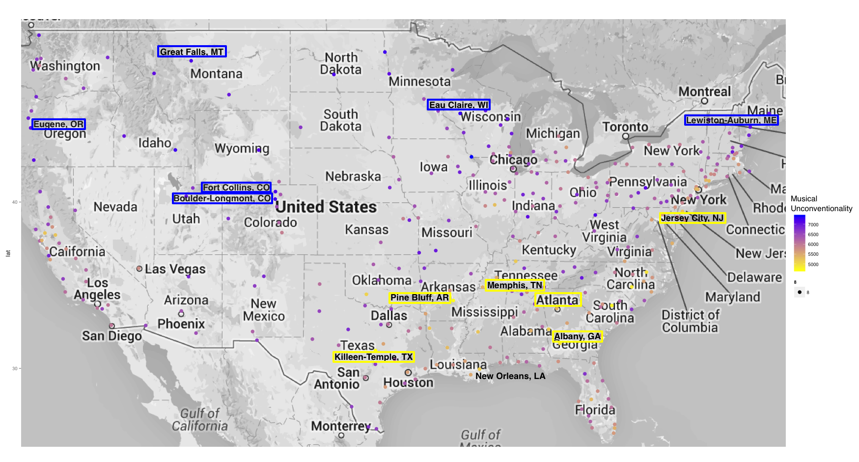
You may also view this list of metropolitan regions in descending order of unconventionality.
But it appears clear from the maps that musical un/conventionality does not align according to a clear geographical pattern. So we run a number of analyses to discover whether musical creation correlates to some metro level demographic variables.
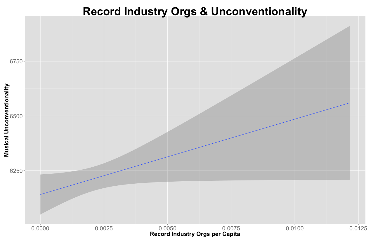
An advantage of aggregating to metro areas is that we can make use of the extensive information we know about them from the U.S. Census Bureau. We draw on two main sources. First is the decennial census, which tells us about demographics. We use total population, percent African-American, percent Hispanic, percent college students, and median household income. Second is Zip Code Business Patterns, which can tell us about a metro’s organizational make-up. For our analysis we focused on organizations related to the music industry: specifically we made a recording industry per capita variable (the total “Record Production,” “Music Publishers,” “Sound recording studios,” and “Other Sound Recording Studios” per person), and also a radio stations per capita variable. These are both based on NAICS codes. Though one might consider many other variables (and we did explore others), given that our N drops precipitously when we move to metros (from three million to three hundred) we try to stick to a small number to avoid collinearity problems. To continue to pursue the relationship between popularity and conventionality now at the aggregate level, we also include the metro median of our band popularity index.
Here are simple bivariate correlations between these variables and a metro area’s median conventionality score.
| Metro Median Unconventionality | Sig. (2-tailed) | |
|---|---|---|
| Total Population | -.200** | <.001 |
| Radio Stations Per Capita | .244** | <.001 |
| Recording Industry Organizations Per Capita | 0.105 | 0.056 |
| Percent African American | -.678** | <.001 |
| Percent College Students | .233** | <.001 |
| Median Household Income | -0.049 | .37 |
| Percent Hispanic | 0.092 | .095 |
| Metro Median Popularity | .294** | <.001 |
| ** Correlation is significant at the 0.01 level (2-tailed). |
And here are results from a simple multivariate OLS regression, showing standardized Beta coefficients and p-values.
| Beta | Sig. | |
|---|---|---|
| (Constant) | <.001 | |
| Total Population | 0.02 | 0.679 |
| Radio Stations Per Capita | 0.135 | 0.002 |
| Recording Industry Organizations Per Capita | 0.099 | 0.021 |
| Percent African American | -0.691 | <.001 |
| Percent College Students | 0.125 | .002 |
| Median Household Income | -0.17 | <.001 |
| Percent Hispanic | -0.102 | 0.016 |
| Metro Median Popularity | 0.092 | 0.034 |
| Dependent Variable: Metro Median Conventionality |
Variables that correlate positively with metro-level unconventionality: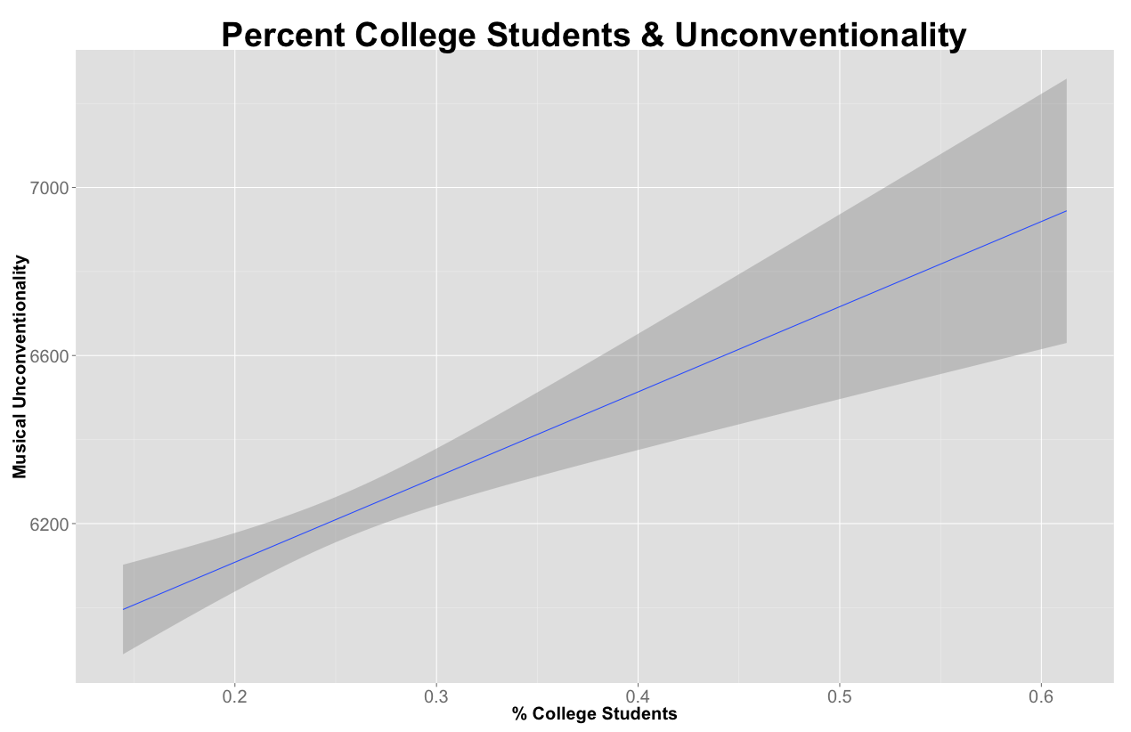

Variables that correlate negatively with unconventionality:

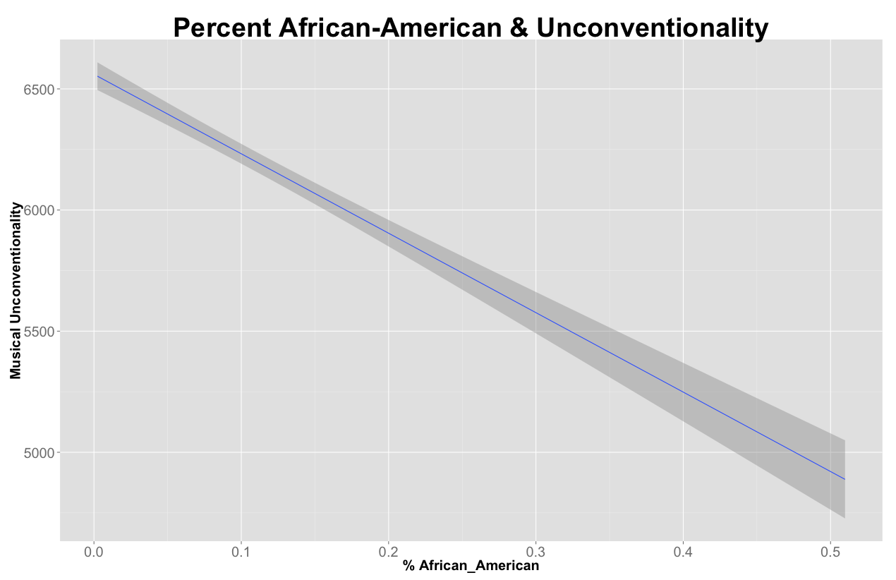
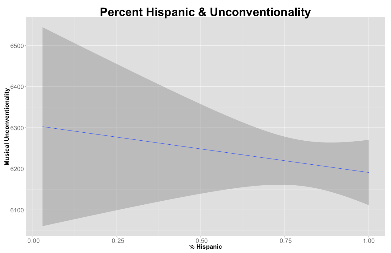
The takeaway is that the most unconventional metros tend to have lots of college students, radio stations, and a strong recording industry presence. By contrast, America’s major popular music clusters are anchored in higher income, more racially diverse (African-American and Hispanic) metros. Interestingly, musically unconventional metros also tend to be home to relatively popular bands. So in contrast to what we saw at the individual band level, at the aggregate level, popularity and unconventionality seem to go together. This raises all sorts of interesting questions, and the interplay between individual band and aggregate metro characteristics is an area we would like to pursue further. Note also finally that total population is insignificant – this too is interesting in that one might have thought that size itself would breed unconventionality (cf. Simmel’s “Metropolis and Mental Life”), but this does not seem to be the case. It also provides some evidence against the possible criticism that we’re getting higher unconventionality scores for smaller metros only due to the tendency of smaller populations to yield extreme values (cf. Gelman).
And now we return to where we started, with the Boss’s speech. We found little support for his idea that American popular musicians freely roam across genres; they mostly operate according to what seem to be strong conventions about what genres go together. But not everywhere to the same degree. Indeed, if we conjure a picture of the Austin SxSW crowd, it looks a lot like the regression results: college students, radio stations, and the record industry. While America in general may not conform to the Springsteen Hypothesis, in some contexts it comes closer than others, and Austin is probably one of them. Considered in this way we might take Springsteen’s speech less as a general proposition and more as a specific expression of the expectations he and his audience have about the nature of musical creativity, one which is by no means universally shared. In other words, he was preaching to the choir.
Certainly these last ideas are speculative, but we hope to pursue them along a number of fronts. We mentioned some above: multi-level analysis that simultaneously investigates metro properties, band properties, and their interactions; diving deeper into the positions of specific genres within the network structure; investigating other variables. Another idea is to (somehow) transform the seventeen clusters into variables, so we can determine their relative strength across (geographic) space. And we might try matching the data to other geographies, such as counties.
But for now, that is all. We would love to hear any comments you may have. Thanks.