If you follow me on Twitter, you know that I’m a big fan of RuPaul’s Drag Race. The transformation, the glamour, the sheer eleganza extravanga is something my life needs to interrupt the monotony of grad school. I was able to catch up on nearly four seasons in a little less than a month, and I’ve been watching the current (fifth) season religiously every Monday at Plan B, the gay bar across from my house.
I don’t know if this occurs with other reality shows (this is the first I’ve been taken with), but there is some element of prediction involved in knowing who will come out as the winner. A drag queen we spoke with at Plan B suggested that the length of time each queen appears in the season preview is an indicator, while Homoviper’s “index” is largely based on a more qualitative, hermeneutic analysis. I figured, hey, we could probably build a statistical model to know which factors are the most determinative in winning the competition.
If you’ve never seen the show, here’s the deal: anywhere from 9 to 13 contestants start the season, selected from a large pool of aspiring drag queens. Every episode, the queens participate in two challenges: a mini-challenge and a main challenge. The mini-challenge is usually some small scale task (dressing up a doll in drag, lipsyncing to one of RuPaul’s songs). The winner(s) of these challenges get some sort of leg up into some part of the main challenge. The main challenge usually has some performative and/or creative element (dancing, singing, making an outlandish costume out of mundane items), which is often combined with a runway performance. At the end of the show, one queen wins, while two are “up for elimination” and forced to “lipsync for their lives.” In dramatic fashion, the queens attempt to outdo one another by lipsyncing to a song they’ve prepared for the week. RuPaul then allows one queen to stay and forces one to “sashay away” (although note that there has been one “double elimination” in the current season when both queens performed subpar, and sometimes Ru lets both queens stay). The judges also note who came close to winning and who came close to being forced to lipsync.
The (Super)model (of the world)
Taking some inspiration from Brett Keller’s Hunger Games post, I figured that a survival analysis (also called event history analysis) would be the best suited for this task. Survival analysis attempts to model which elements are the most determinative in having an impact on the duration of “survival.” I’ve never really delved into the world of survival analysis so I spent the last month reading up with Box-Steffensmeier and Jones’s excellent book. Survival coefficients can be read as impacting the “hazard rate” — the rate at which units “fail” — usually denoted as h(t) (hence the title of this post). As is most common nowadays, I used a Cox proportional hazard model given that it is a semiparametric method and you don’t have to make assumptions about the shape of the distribution of hazard rates (like the Weibull and Gompertz models).
As per standard practice for survival analysis, the dependent variable is “duration” or the length of time that the unit stays alive. For Drag Race, this is the number of episodes that the queen stays on the show. There is a set of covariates that I’ve decided may have potential predictive power. These covariates fall into two classes — time-invariant and time-variant. There may be others, but I’ll discuss those more at the end of this article.
Time-invariant covariates
These variables are ones that we can get before the season even starts. If they turn out to be significant then it might give us some insight into forecasting how the season will go before it even starts.
- Age – The queens who’ve participated on RuPaul’s Drag Race have been anywhere between 21 and 39 years old. Like any performance-based form, the quality of one’s drag usually gets better with age. However, you could also argue that being a better drag queen is highly contingent on having a youthful look and being able to muster a young demeanor. There’s been some animosity between young and old queens (e.g. 37-year old Coco Montrese calling the 21-year old Serena ChaCha a “little boy”), but it’s not clear if there’s an impact of age on actually winning the competition.
- Plus size – Every season has had at least one “plus size” queen. These “big girls” have generally not gone far in the competition. The furthest any one has gotten has been Latrice Royale, who placed 4th in season 4. There’s also a healthy amount of “fat-phobia” from other queens. I’m throwing this in to see if there is any sort of plus size penalty.
- Puerto Rican – Along with being a big girl, each season has had at least one Puerto Rican queen. I chose to focus on Puerto Rican as a variable instead of race/ethnicity more generally because the Puerto Rican queens often come up against a challenge with language and participating in particular challenges that require more linguistic nuance and humor. That said, while none of these queens have ever taken the crown, they often have gotten very far — Nina Flowers placed 2nd in Season 1 and Alexis Mateo placed 3rd in season 3.
Time-variant covariates
These variables change as the season goes on. They serve as indicators of the queen’s performance throughout the competition.
- Wins – Winning a main challenge is a pretty big deal. It generally earns the queens respect amongst the judges and the other queens. It makes a bit of sense that a queen with a consistent track record of winning challenges will generally stay on the show longer.
- Lipsyncs – “Lipsyncing for your life” is a generally harrowing affair. It is the last chance to impress RuPaul, so the queens better make it good. Having to lipsync is the opposite of a win — it looks bad to the judges and to the other queens, and shakes one’s own confidence.
- Highs and lows – Apart from actually winning challenges or having to lipsync, the judges will also note whether the queen was in the top or the bottom of the pack but (un)fortunately was not great/mediocre enough to merit any more notice.
I should say a word about the actual “lipsync” variable. I’ve been going back and forth on whether to calculate that variable based on the raw number of lipsyncs (excluding the final one that judges the season winner) or to use one that only includes lipsyncs which do not result in eliminating the contestant. In the models below, I play around with both.
I compiled the data from the detailed Wikipedia charts for each season of the show and put them into a public Google doc. You can access the Google doc as a comma-separated value file as well for easy data wrangling. There’s a row for each contestant and each episode.
The main challenge (now don’t f*$k it up!)
First thing is to load the data. Thanks to the RCurl, I can pull this straight from the Google Doc into R. I’ll also load the survival package and ggplot2 for some plots. I’m also training the model on the first four seasons and am saving the fifth season for the out-of-sample prediction. (To make this post less noisy and more pretty I’m putting most the R code in this gist rather than posting it inline).
Before estimating the Cox model, I want to start with looking at a few univariate analyses for things that may be important predictors. The y-axis on these graphs is the survival rate, while the x-axis represents time measured in episodes. The closer the different strata are to each other, the more similar they are to the effect they have on the survival rate. Because I like pretty ggplot2 graphs I rigged up a function to convert the Survival fit object to something that it could use, with a heavy amount of help from this pdf from Ramon Saccilotto of the Basel Biometric Section.
Age
First, let’s look at age. To make the graph a little cleaner, I’m put age into three strata — less than 25 (coded 1), 25 through 30 (coded 2), and greater than 30 (coded 3). Each of these strata has roughly the same number of queens in it.
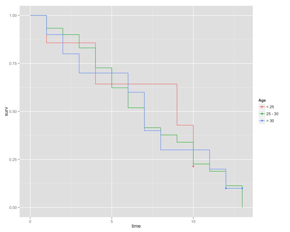
We actually don’t see any major differences between the age strata. Their survival rates seem to decline together, with a slight advantaged gained by the young’ins.
Wins
Turning to the time-variant covariates, let’s look first at the number of main challenges each queen won, and then the number of times that she lipsynced.
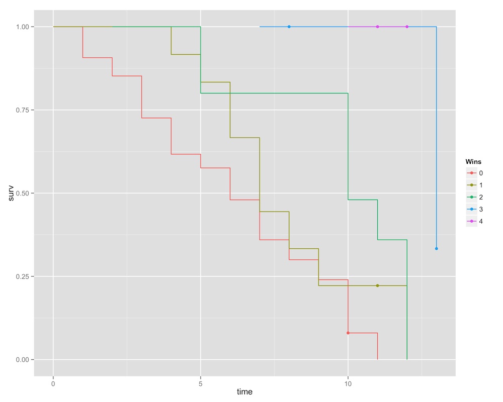
This image is pretty stark. If the queen has won four challenges, she is guaranteed to win (to date, only the great Sharon Needles has accomplished such a feat). Winning three challenges will take you a great deal of the way, but this all changes very late in the game. This graph shows the tense competition of season three, when all three finalists (Raja, Manila Luzon, and Alexis Mateo) had three wins under their… um, petticoats? by the final episodes. Below that, having two wins bodes better, but not much better, than have zero or one.
Lipsyncs
The last graph we look at is lipsyncs.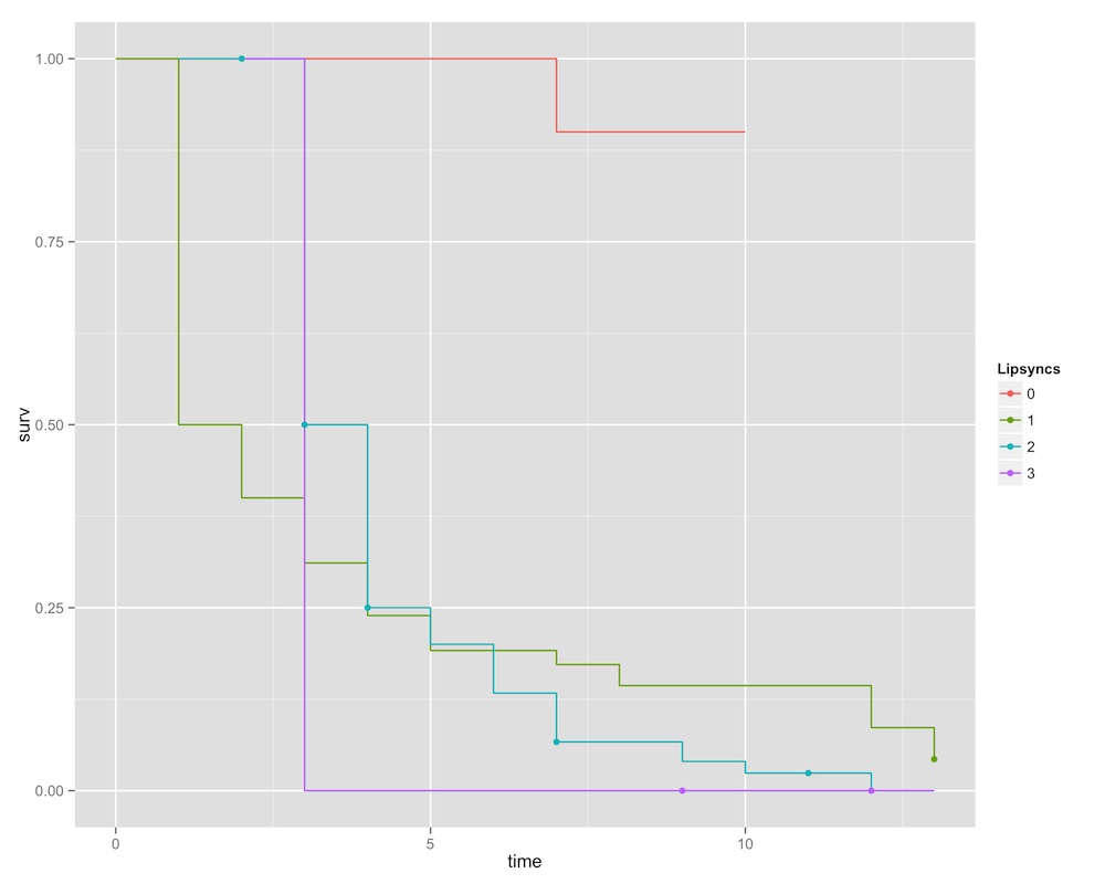
This one is also rather dramatic. With no lipsyncs, chances don’t drop very dramatically. To date, there are only two queens — Nina Flowers and Tyra Sanchez — who have managed to never lipsync. Survival rates drop off perspicaciously after that, however. Contestants can almost guarantee that they will have to sashay away if it’s their third time in the bottom two.
Now for the models. I’m going to start by considering only the time invariant models. If there is some stable pattern that emerges there, then it may be possible to get some purchase on who the next drag superstar will be before the season begins.
Call:
coxph(formula = t.surv ~ (Age + PlusSize + PuertoRico), data = df)

  n= 314, number of events= 41

               coef exp(coef) se(coef)      z Pr(>|z|)
Age        -0.03656   0.96410  0.03262 -1.121   0.2623
PlusSize    0.89174   2.43938  0.44215  2.017   0.0437 *
PuertoRico -0.29471   0.74475  0.44815 -0.658   0.5108
---
Signif. codes:  0 '***' 0.001 '**' 0.01 '*' 0.05 '.' 0.1 ' ' 1

           exp(coef) exp(-coef) lower .95 upper .95
Age           0.9641     1.0372    0.9044     1.028
PlusSize      2.4394     0.4099    1.0255     5.803
PuertoRico    0.7448     1.3427    0.3094     1.793

Concordance= 0.592  (se = 0.058 )
Rsquare= 0.014   (max possible= 0.542 )
Likelihood ratio test= 4.48  on 3 df,   p=0.2142
Wald test            = 4.79  on 3 df,   p=0.1876
Score (logrank) test = 4.96  on 3 df,   p=0.1746
This model does not seem to hold up very well on the whole. The LR and Wald tests don’t let us reject the hypothesis that all of the coefficients are equal to zero. The only variable that turns up as statistically significant is plus size. Being a big girl increases her hazard rate by a factor of 2.43 on average, or 143%. The model also shows weak effect sizes for age and the Puerto Rican cases. Age goes in the direction we expected, but being Puerto Rican does not. It actually reduces the hazard rate.
So that model isn’t terribly helpful. Let’s start to incorporate time variant covariables. First, I include all time invariant covariants and add the time variant covariates. Note, to account for temporal dependence between observations, I’ve included the cluster term which produces robust standard errors, which is what Box-Steffensmeier and Jones advise.
Call:
coxph(formula = t.surv ~ (Age + PlusSize + PuertoRico + Wins +
    Highs + Lows + Lipsyncs) + cluster(ID), data = df)

  n= 314, number of events= 41

                coef exp(coef)  se(coef) robust se      z Pr(>|z|)
Age        -0.005792  0.994225  0.044982  0.037835 -0.153    0.878
PlusSize    0.186822  1.205413  0.487592  0.542285  0.345    0.730
PuertoRico -0.465269  0.627966  0.615109  0.695995 -0.668    0.504
Wins       -0.210350  0.810300  0.328441  0.369647 -0.569    0.569
Highs       0.269315  1.309067  0.290462  0.339070  0.794    0.427
Lows        0.100976  1.106250  0.456684  0.548226  0.184    0.854
Lipsyncs    1.436659  4.206618  0.302593  0.319964  4.490 7.12e-06 ***
---
Signif. codes:  0 '***' 0.001 '**' 0.01 '*' 0.05 '.' 0.1 ' ' 1

           exp(coef) exp(-coef) lower .95 upper .95
Age           0.9942     1.0058    0.9232     1.071
PlusSize      1.2054     0.8296    0.4164     3.489
PuertoRico    0.6280     1.5924    0.1605     2.457
Wins          0.8103     1.2341    0.3926     1.672
Highs         1.3091     0.7639    0.6735     2.544
Lows          1.1062     0.9040    0.3777     3.240
Lipsyncs      4.2066     0.2377    2.2469     7.876

Concordance= 0.882  (se = 0.058 )
Rsquare= 0.17   (max possible= 0.542 )
Likelihood ratio test= 58.43  on 7 df,   p=3.1e-10
Wald test            = 104.6  on 7 df,   p=0
Score (logrank) test = 72.23  on 7 df,   p=5.226e-13,   Robust = 33.47  p=2.167e-05

  (Note: the likelihood ratio and score tests assume independence of
     observations within a cluster, the Wald and robust score tests do not).
This model does much better compared to the first model. LR and Wald tests allow us to reject the null that all coefficients are not different from zero. Lipsyncs here come out as the most obvious predictor. The effect is large and highly statistically significant. On average, an additional lipsync will increase a queen’s hazard rate by a factor of 4.21 — 321%! Lipsyncing has a huge penalty, hunty. It doesn’t bode well for winning the crown.
But maybe we are overfitting. Lipsyncing is the only thing that can knock a queen out of the contest (except if the queen is Willam Belli, who was disqualified for breaching the show’s contract). It may be possible that it has such close correlation with the instance of the event that we’re losing more nuanced trends in the data. For this fact, I calculated a variable that counted the number of lipsyncs excluding those instances in which it knocked the queen out of the contest and replaced the existing lipsync variable with it.
Call:
coxph(formula = t.surv ~ (Age + PlusSize + PuertoRico + Wins +
    Highs + Lows + LipsyncWithoutOut) + cluster(ID), data = df)

  n= 314, number of events= 41

                      coef exp(coef) se(coef) robust se      z Pr(>|z|)
Age               -0.04716   0.95393  0.04104   0.04040 -1.167 0.243043
PlusSize           0.10505   1.11076  0.49714   0.56345  0.186 0.852102
PuertoRico        -0.07008   0.93232  0.48455   0.39676 -0.177 0.859791
Wins              -1.13417   0.32169  0.28403   0.22578 -5.023 5.08e-07 ***
Highs             -0.63124   0.53193  0.21924   0.18725 -3.371 0.000749 ***
Lows              -1.17747   0.30806  0.37894   0.36645 -3.213 0.001313 **
LipsyncWithoutOut -0.07052   0.93191  0.26342   0.26588 -0.265 0.790835
---
Signif. codes:  0 '***' 0.001 '**' 0.01 '*' 0.05 '.' 0.1 ' ' 1

                  exp(coef) exp(-coef) lower .95 upper .95
Age                  0.9539     1.0483    0.8813    1.0325
PlusSize             1.1108     0.9003    0.3681    3.3514
PuertoRico           0.9323     1.0726    0.4284    2.0290
Wins                 0.3217     3.1086    0.2067    0.5008
Highs                0.5319     1.8799    0.3685    0.7678
Lows                 0.3081     3.2462    0.1502    0.6318
LipsyncWithoutOut    0.9319     1.0731    0.5534    1.5692

Concordance= 0.713  (se = 0.058 )
Rsquare= 0.093   (max possible= 0.542 )
Likelihood ratio test= 30.82  on 7 df,   p=6.712e-05
Wald test            = 41.27  on 7 df,   p=7.188e-07
Score (logrank) test = 32.46  on 7 df,   p=3.333e-05,   Robust = 24.62  p=0.0008875

  (Note: the likelihood ratio and score tests assume independence of
     observations within a cluster, the Wald and robust score tests do not).
With this model, we lose some explanation in terms of variance (R-squared goes from 0.17 to 0.093), but three variables — wins, highs, and lows — gain statistical significance. Wins and highs go in the expected direction: for each additional win or high, the hazard rate decreases by a factor of 3.11 and 1.88, respectively. But, oddly enough, for each additional low, the hazard rate decreases by a factor of 3.25! That doesn’t really seem right. It may be that what’s happening is that those queens who accumulate low judging are still “safe” but aren’t getting into any real trouble.
So it may be that the original lipsync variable is a better model. A little toying with some k-fold-like validation in which I train the model on the first three seasons and predict the fourth season (not shown, saving it for next week) says that it seems like a better model.
The future of drag!
This is a rough first attempt at quantifying the sheer sickening amount of glamour that RuPaul provides. There are three outstanding topics to address — prediction, repeated events, and where to get more data.
Using the predict.coxph() function included in the survival package, we can compute the relative risks of the remaining queens in season 5 (this StackOverflow article has a nice explanation of what this function does. Thanks to Trey for pointing this out). I’m using the second model, with the full lipsync count.
            Name   relRisk se.relRisk
1 Alyssa Edwards 0.2931656  0.1887553
2  Jinkx Monsoon 0.6226868  0.3119846
3 Roxxxy Andrews 0.6691839  0.6217982
4    Ivy Winters 0.6809134  0.6087346
5         Alaska 0.7060275  0.5789992
6          Detox 1.1475463  0.5733333
7  Coco Montrese 5.6221514  1.4578057
The model has Coco Montrese down, which makes sense: one more lipsync and she’s up to three, meaning she has nearly no chance of staying in the race. Detox is the only other contestant that’s lipsynced this season so she’s not looking great either unless she pulls a win soon. Judging from the standard errors, Roxxxy, Ivy, and Alaska may bounce … around a bit. Alyssa and Jinkx look unusually strong. Homoviper’s latest analysis projections look a bit different: Ivy, Jinkx, Alaska, Alyssa, Roxxxy, Detox, and finally Coco. In next week’s post, I’ll focus more on exploring prediction.
Another concern is that of repeated events. Given that in the last two seasons, Ru has brought back one queen who had been previously eliminated, there’s no reason to suspect that she won’t do it again. So far I’ve dealt with it by only counting a queen’s final exit. But this may be biasing the model in unexpected ways. One obvious way to treat this is a case of repeated events. There are a number of methods for treating repeated events but I’m not terribly familiar with them.
Lastly, there are other sources of data that we could be pulling from. I mentioned the potential of preview appearances, which may indicate a number of things — the amount of airtime that each queen gets, how catty she is, etc etc. But they at least need enough footage to do so. I did a rough count from this season’s trailer and it roughly correlates with the top eight at least. A few other time invariant covariates could include if a queen is a pageant girl and actual time in the drag industry (as opposed to age). Barring a solid measure of fierceness this is what we’ve got to work with.
Anyhow, until next time — if you can’t love yourself, how the hell you gonna love somebody else. Can I get an amen?!
(Thanks a bunch to Martha and Trey for help putting together this post! The former claims 3% authorship on it.)