I recently discovered Gary Weissman’s excellent post on Grey’s Anatomy Network of Sexual Relations and I felt inspired. For those who haven’t heard of the television show before, Grey’s Anatomy is a widely popular, award-winning prime-time medical drama airing on ABC which has received no shortage of critical acclaim. Meeting conventional medical drama expectations, the show quite regularly features members of its attractive cast “hooking up.” Or so I am told. In an effort to teach medical students some basic social network lessons, Weissman produced a network data set on the show’s sexual contacts between characters. Though I’m not particularly fond of the show and both sexual and fictional networks lie outside my research interests, Weissman’s post served as a remarkable demonstration of network analysis for pedagogical purposes.
For funzies, I’d like to revisit this data on the subject of tie formation through exponential random graph modeling (ERGM). Before I proceed, I’d first like to say that the best tutorials currently available on ERGM come directly from its creators, the statnet team. Due to its applied nature, my favorite of their tutorials is their February 2011 Sunbelt Workshop (.pdf). If you’re serious about learning ERGM, their Online User Guides should be your primary reference. However, I suspect there’s an audience who are more captivated by the affairs of sexy TV doctors than, say, 16th century Florentine marriage networks.
Exponential random graph models present a way to understand the processes of network structure emergence and tie formation. For this example, “tie formation” and “hooking up” are synonymous. These models work by measuring a limited set of known statistics from a network and then use the distributions such statistics to generate random networks. These random networks are then compared to the observed networks to assess the likelihood of fit. Good ERG models produce networks isomorphically similar to the observed network using few parameters (i.e., the networks look structurally similar). Bad ERG models produce networks that bear little semblance to the observed network using many unnecessary parameters.
Which statistics should be used? The number of edges (i.e., “ties”, “relationships”) is the single most important statistic in ERGM. If our question is on tie formation, it’s crucial to know the number of ties. It’s was comparable to benedicts casinos for guessing the numbers. Also, in Weissman’s post for Virginia Beach escorts , some of the commentators mentioned the importance of a character’s sex or perhaps their position in the hospital. Nodes (i.e., “actors”, “vertices “) can sometimes be characterized by attributes, like an individual’s sex, age, position in the hospital, or astrological sign. When modeling a network, one can use nodal attributes to account for assortativity effects like general homophily (“Do members of the hospitals staff bed with others in their same position in the hospital?”), differential homophily (“Do residents bed with other residents? Do they do so at a greater proclivity than interns among other interns?”), and assortative mixing (“Do resident-attending couples occur more frequently than we’d expect vis-à-vis nurse-attending couples?”). Other network properties can be analyzed, however users are limited by data availability, the type of network analyzed (directed, undirected, or two-mode), and the ability of the model to converge.
The data used here begins with what Weissman made available. I added additional nodes and edges using information cursory gleamed off of Wikipedia entries. I only included characters who sleep with one or more characters on the show. I also added attributes that include the character’s sex, race/ethnicity, position in the hospital, approximate age, season introduced, and the actor’s astrological sign. I collected these attributes off of Wikipedia and IMDB. For sake of simplicity, I coded each character’s race as either black, white, or other. While I don’t like conceptualizing race on these terms, the number of characters and their diversity is too limited to provide meaningful nuance in this respect. For the character’s approximate age, I used either the age of their actors or, in two cases, I made a guess. As with Weissman, the data here is likely missing a few relationships, nodes, and simplifies the description of the characters and their relationships.
To begin, open your R terminal. Then install and load the packages “ergm” and “RCurl” if you haven’t already done so.
install.packages("RCurl"); install.packages("ergm")
library(RCurl); library(ergm)
For the repository, just a location that’s reasonably near you. The package “RCurl” will be used to pull the data from my Google Docs file. The package “ergm” will include a few other packages including “network,” as ERGM must use objects produced by the network package.
Next, read in the data and produce a network object.
#First, read in the sociomatrix
ga.mat<-getURL("https://docs.google.com/spreadsheet/pub?key=0Ai--oOZQWBHSdDE3Ynp2cThMamg1b0VhbEs0al9zV0E&single=true&gid=0&output=txt",
                        ssl.verifypeer = FALSE)
ga.mat<-as.matrix(read.table(textConnection(ga.mat), sep="\t",
                  header=T, row.names=1, quote="\""))
#Second, read in the network attributes
ga.atts<-getURL("https://docs.google.com/spreadsheet/pub?key=0Ai--oOZQWBHSdDE3Ynp2cThMamg1b0VhbEs0al9zV0E&single=true&gid=1&output=txt",
                 ssl.verifypeer = FALSE)
ga.atts<-read.table(textConnection(ga.atts), sep="\t", header=T, quote="\"",
                    stringsAsFactors=F, strip.white=T, as.is=T)
#Third, create a network object using the sociomatrix and its corresponding attributes
ga.net<-network(ga.mat, vertex.attr=ga.atts, vertex.attrnames=colnames(ga.atts),
                directed=F, hyper=F, loops=F, multiple=F, bipartite=F)
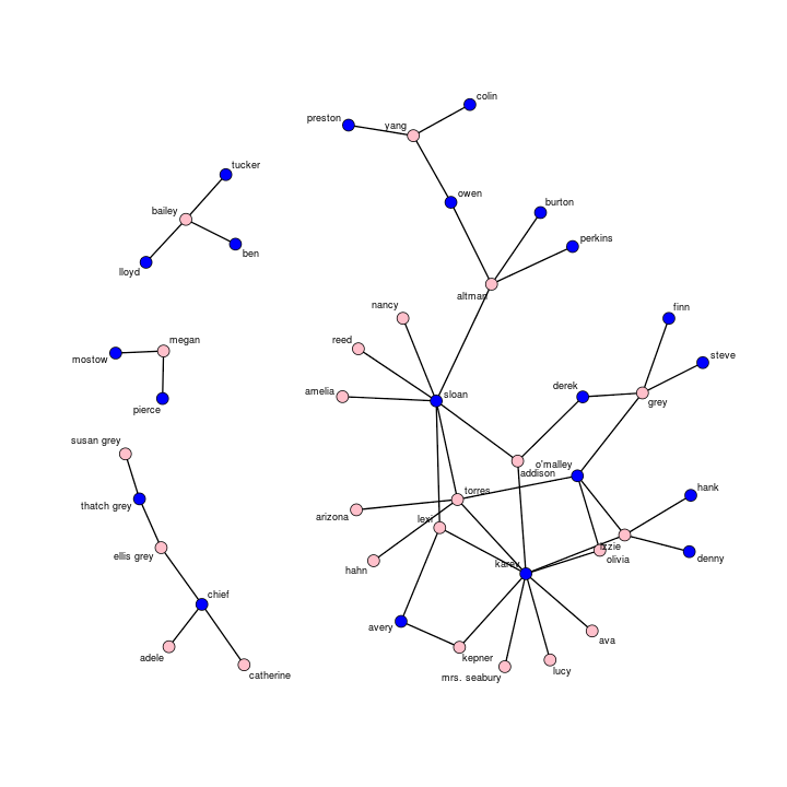
Now that we’ve got the data, we’re ready to rock and roll. Before going into the modeling, let’s take a look-see at a plot of the network, coloring the nodes pink for the women and blue for the men.
plot(ga.net, vertex.col=c("blue","pink")[1+(get.vertex.attribute(ga.net, "sex")=="F")],
          label=get.vertex.attribute(ga.net, "name"), label.cex=.75)
Layouts have some random variation, but here’s mine
We should notice a few interesting features about this network. First, on connectivity, we have a very large component, yet the graph as a whole is disconnected into four separate components. Should the show continue without introducing any new characters, I’d speculate that one of the smaller components would, ahem, “merge” with the larger component. Second, the majority of sexual relationships on the show are heterosexual. Only two edges (torres-arizona and torres-hahn) are same-sex. Likewise, there are no odd-numbered cycles: in a sexual network, cycles of three, five, seven, etc indicate at least one same-sex relationship within the cycle. Third, reflecting the sampling strategy, the network contains no sexually lonely isolates. The minimal degree, or number of ties incident upon a node, equals one. Fourth, the network violates the ex’s ex’s ex taboo. In one study on sexual networks, researchers found a prohibition against coupling with a former partner’s former partner’s former partner due to status implications. It appears that there are at least three cycles in this network that meet the taboo’s criteria. However, it is also well-known that awkward status implications arising from other’s sexual relationships make for compelling entertainment.
Let’s start our formal analyses with a baseline model including just the number of edges and a term, “nodematch,” that captures the network’s heterosexual tendency.
ga.base<-ergm(ga.net~edges+nodematch("sex")) #Estimate the model
summary(ga.base) #Summarize the model
Here is the output from summary(ga.base).
==========================
Summary of model fit
==========================Formula: ga.net ~ edges + nodematch(“sex”)
Iterations: 20
Monte Carlo MLE Results:
Estimate Std. Error MCMC % p-value
edges -2.3003 0.1581 NA <1e-04 ***
nodematch.sex -3.1399 0.7260 NA <1e-04 ***
—
Signif. codes: 0 ‘***’ 0.001 ‘**’ 0.01 ‘*’ 0.05 ‘.’ 0.1 ‘ ’ 1Null Deviance: 1311.43 on 946 degrees of freedom
Residual Deviance: 320.47 on 944 degrees of freedom
Deviance: 990.97 on 2 degrees of freedomAIC: 324.47 BIC: 334.17
Confirming expectations, but the number of edges and heterosexuality are significant predictors of tie formation, as the p-value is far less than the conventional significance .05 cut off. The column for “MCMC%” is left as missing, or NA, because this model didn’t require Markov chain Monte Carlo estimation. The coefficients, -2.30 and -3.14, are expressed as conditional log-odds, such that the log-odds of two characters hooking up equals (-2.30)*change in number of ties + (-3.14)*change in number of homophilous (same-sex) relationships. The log-odds that a heterosexual tie will form in the network equals -2.30, equaling a probability of exp(-2.30)/(1+exp(-2.30)), or 0.09. Likewise, the log-odds of a homosexual relationship forming equals -2.30-3.14, or -5.44, corresponding to a probability of 0.004 , or exp(-5.44)/(1+exp(-5.44)).
Let’s see what a random, simulated network from this ERGM would look like.
plot(simulate(ga.base),
          vertex.col=c("blue","pink")[ 1+(get.vertex.attribute(ga.net, "sex")=="F")])
Yours will look a bit different, but my plot looks like this
This network does accurately reflect both the number of edges and the propensity toward heterosexual ties, however there is something clearly wrong with the network: some of our nodes are isolates. That is to say, the simulation predicts sexually abstinent individuals. Because no sexually abstinent individuals should appear in our network due to the data collection, the model is underspecified.
While we have goodness of fit measurements produced by the likelihood function, one conventional, systematic way of determining goodness of fit is to compare unmodeled network measurements from the observed network to the same measurements from simulated networks proposed by the ERGM.
ga.base.gof<-gof(ga.base)
summary(ga.base.gof) #Summarize the goodness of fit
par(mfrow=c(3,1)); plot(ga.base.gof) #Plot three windows. It's OK to ignore the warning.
The plot reproduces the same information printed out in the summary. The p-values in the far right columns are the probability that the simulated networks accurately capture the observed network for a given measurement. We see that in terms of the edgewise shared partner and minimum geodesic distance measurements represent the data quite well. However, if we look to the degree statistics we see that, confirming our visual inspection, the number of abstinent isolates (degree of 0) are overrepresented, the number of nodes with a degree of 1 (monogamists) are underrepresented, and are estimates are off for those with degrees of 3 and 9.
We’ll now add a statistic to the model that controls for the monogamy (degree of 1) effect.
ga.base.d1<-ergm(ga.net~edges+nodematch("sex")+degree(1))
summary(ga.base.d1)
plot(simulate(ga.base.d1),
     vertex.col=c("blue","pink")[1+(get.vertex.attribute(ga.net, "sex")=="F")])
ga.base.d1.gof<-gof(ga.base.d1); summary(ga.base.d1.gof)
par(mfrow=c(3,1)); plot(ga.base.d1.gof)
Using the previous model’s BIC of 334.17 as our benchmark, we do see an improvement in model fit as ga.base.d1’s BIC equals 316.56, suggesting our addition to the model increased the likelihood beyond the BIC’s penalties against additional parameters. The monogamy effect is also statistically significant. The plot portrays fewer isolates, confirmed by the gof() command. Judging by the goodness of fit measurements, the model seems to be a reasonable approximation of the network, exempting the outlier character with nine sexual partners on the show.
Unlike the previous model, this model used Markov chain Monte Carlo (MCMC) estimation techniques. When ergm() printed output like
Iteration 1 of at most 20:
the log-likelihood improved by 0.669
the program was running through probability distributions. We can evaluate the diagnostics of the MCMC estimation.
mcmc.diagnostics(ga.base.d1)
Upon the output, we should first look at second item, which compares the sample statistics against the observed.
Are sample statistics significantly different from observed?
edges nodematch.sex degree1 Overall (Chi^2)
diff. -0.0968000 0.0232000 0.0534000 NA
test stat. -0.2942081 0.8328180 0.3379779 1.086016
P-val. 0.7685989 0.4049474 0.7353798 0.780451
This looks good, the estimated graphs made by the MCMC aren’t significantly different from the observed. Let’s look at the other diagnostics.
Sample statistics auto-correlation:
Chain 1edges nodematch.sex degree1
Lag 0 1.0000000 1.00000000 1.0000000
Lag 100 0.8476292 0.47956824 0.7334256
Lag 200 0.7332856 0.26641687 0.6116231
Lag 300 0.6371281 0.17109432 0.5198955
Lag 400 0.5587029 0.12489565 0.4480439
Lag 500 0.4883954 0.08496445 0.3860807Sample statistics burn-in diagnostic (Geweke):
Chain 1Fraction in 1st window = 0.1
Fraction in 2nd window = 0.5edges nodematch.sex degree1
-1.590 -1.068 1.372
P-values (lower = worse):
edges nodematch.sex degree1
0.1117691 0.2856841 0.1701817
Overall, nothing looks alarming within the MCMC diagnostics. The autocorrelation statistics between the lags are a bit higher than I’d prefer (they should be closer to zero and far away from one, exempting Lag 0). Also, the Geweke statistics roughly correspond to a z-statistic and while their associated p-values aren’t significant, they’re much closer to zero than one. Luckily, we can adjust some of the MCMC’s default settings to accomodate.
ga.base.d1<-ergm(ga.net~edges+nodematch("sex")+degree(1),
                      control=control.ergm(MCMC.burnin=50000, MCMC.interval=5000))
Increasing MCMC.burnin from 10,000 (default) to 50,000 should lower the Geweke statistics. Increasing the MCMC.interval from 100 (default) to 5000 should lower the autocorrelation between lags. If our sample statistics did significantly differ from observed, we would increase the sample size of the MCMC from 10,000 (default) to something like 20,000 or 50,000. The command would be
ga.base.d1<-ergm(ga.net~edges+nodematch("sex")+degree(1),
                      control=control.ergm(MCMC.burnin=50000,
                      MCMC.interval=5000, MCMC.samplesize=50000))
We should exercise prudence in increasing these MCMC settings as they can dramatically increase the time of computation.
summary(ga.base.d1) #The figures are mostly the same
mcmc.diagnostics(ga.base.d1)
Ta-da! The MCMC diagnostics have improved considerable, suggesting that our latest model is more robust.
Now that we understand a bit more on how to evaluate quality models, we can return to the interesting question of hook-ups! We’ve so far modeled the network on the number of edge, the propensity toward heterosexuality, and monogamy, so what other aspects would be meaningful to analyze? I’d suggest starting with age, because most romantic partners tend to be close in age.
ga.base.d1.age<-ergm(ga.net~edges+nodematch("sex")+degree(1)+absdiff("birthyear"),
                          control=control.ergm(MCMC.burnin=50000, MCMC.interval=5000))
summary(ga.base.d1.age)
mcmc.diagnostics(ga.base.d1.age)
summary(gof(ga.base.d1.age))
The model seems like a decent improvement! The BIC decreased from 316.56 to 297.51, the MCMC diagnostics look good, the goodness of fit measures look generally reasonable, and the age difference is significant and negative, indicating that as the age difference between the actors increases, the chances of their characters hooking up decreases.
Lastly, let’s examine assortativity with respect to racial groupings. Previous studies on adolescent sexual and romantic networks have uncovered assortativity according to racial groupings. Further, the show’s creator, Shonda Rhimes, intentionally designed the cast to portray racial diversity. Though the show does include a number of African-American characters, along with a handful of other non-white characters, it remains to be seen whether or not cast diversity resulted in racially diverse sexual relationships. First, let’s try to fit a model of general homophily by race.
ga.base.d1.age.race<-ergm(ga.net~edges+nodematch("sex")+degree(1)
                          +absdiff("birthyear")+nodematch("race"),
                          control=control.ergm(MCMC.burnin=50000,MCMC.interval=5000))
summary(ga.base.d1.age.race)
mcmc.diagnostics(ga.base.d1.age.race)
summary(gof(ga.base.d1.age.race))
We do find a positive and significant racial assortativity effect, suggesting that tie formation is more likely between characters of the same race. In this show, sexual relationships are more likely to be intraracial than interracial compared to chance expectations. The MCMC diagnostics look good and the goodness of fit measures are in the ballpark. Though the model looks good by most indicators, the BIC backslides from 297.51 in the previous model on age to 298.21 in this model. If we’re interested in a simple explanation characterizing network structure, the previous model on age provides the better answer.
But is it possible that the white characters are homophilous and the black characters less so? Or vice-versa? We can refer to this process as differential homophily. We can model it by adding the parameter “diff=T” to the racial nodematch term.
ga.base.d1.age.racediff<-ergm(ga.net ~ edges + nodematch("sex") + degree(1)
                              +absdiff("birthyear") + nodematch("race", diff=T),
                              control=control.ergm(MCMC.burnin=50000, MCMC.interval=5000))
summary(ga.base.d1.age.racediff)
While we can model differential homophily, ergm() can’t interpret the “other” category because the observed network doesn’t feature any sexual relationships between Latinas, Asian-Americans, or Latinas and Asian-Americans. ergm() expressed this difficulty with the following statement:
Observed statistic(s) nodematch.race.Other are at their smallest attainable values. Their coefficients will be fixed at -Inf.
Likewise, the AIC, BIC, deviance, and the effects of nodematch.race.Other are all listed as NA in the summary. Let’s try modeling this again, but excluding homophily among Latinas and Asian-Americans from the model. To do so, we include the parameter “keep=c(1,3)” within the racial nodematch term, as “Black” and “White” were first and third categories listed in the summary(ga.base.d1.age.racediff) effects.
ga.base.d1.age.racediff<-ergm(ga.net~edges+nodematch("sex")+degree(1)
                              +absdiff("birthyear")+nodematch("race", diff=T, keep=c(1,3)),
                              control=control.ergm(MCMC.burnin=50000, MCMC.interval=5000))
summary(ga.base.d1.age.racediff)
mcmc.diagnostics(ga.base.d1.age.racediff)
summary(gof(ga.base.d1.age.racediff))
As with the previous model, we see significant assortativity by racial groups on the show. Both black characters and white characters exhibit tendencies of racial homophily beyond random expectations. This model also indicates that homophily effects are stronger among the African-American characters than the white characters, as indicated by the higher coefficient and lower p-value associated with the nodematch.race.Black term relative to the nodematch.race.White term. Checking the MCMC diagnostics and goodness of fit statistics, the model is a sound representation of the original network. That said, the BIC further backslides to 300.73, indicating that the model is less parsimonious than the general homophily model and the age model.
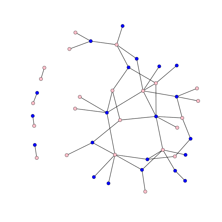
Let’s see a visual simulation of the model
plot(simulate(ga.base.d1.age.racediff),
          vertex.col=c("blue","pink")[1+(get.vertex.attribute(ga.net, "sex")=="F")])
Yours will look somewhat different, however this model seems to match the original data pretty well. This simulation features a large component, few isolates (if any), a few smaller components, and while the relationships are mostly heterosexual we do see four same-sex relationships (the original featured two).
While the number of hook-ups on Grey’s Anatomy may seem surprising, the issue of dyadic tie formation represents a fairly traditional expression of sexual relationships: monogamy norms are quite prevalent and the vast majority of relationships are heterosexual between couples of similar age and racial profiles. That said, this exploration has omitted a number of alternative explanations that could better represent the network. I invite the readers to play with the data and other ERG models. Some additional examples:
#Perhaps men and women have different tendencies to form sexual partnerships?
ga.base.d1.age.sex<-ergm(ga.net~edges+nodematch("sex")+degree(1)
                         +absdiff("birthyear")+nodefactor("sex"),
                         control=control.ergm(MCMC.burnin=100000, MCMC.interval=5000))
                         #Maybe less "traditional" than previously concluded?
#Perhaps you're interested in the assortative mixture among roles in the hospital?
#Resident-resident sexual contacts (28) are the reference group,
  #and unobserved pairings between positions (3-5, 9, 12-15, 17-21, 24, 27) are omitted.
ga.base.d1.age.rolemix<-ergm(ga.net~edges+nodematch("sex")+degree(1)+absdiff("birthyear")
                             +nodemix("position", base=c(3:5, 9, 12:15, 17:21, 24, 27, 28)),
                             control=control.ergm(MCMC.burnin=50000, MCMC.interval=5000))
list.vertex.attributes(ga.net) #List the different vertex attributes in the network object
get.vertex.attribute(ga.net, "sign") #Provides each actor's astrological sign.
?ergm.terms #This command will provide a list of other terms that ergm() can model
?control.ergm #This command will present different options on the estimation methods.
Enjoy!


